In the NFL, quarterback sacks can be game-changing plays that dramatically affect the outcome of games. Understanding the factors that contribute to sacks is crucial for both defensive coordinators looking to pressure opposing quarterbacks and offensive coaches trying to protect their own. This analysis explores the use of logistic regression to predict sack probability on passing plays.
Exploratory Data Analysis
Before building the model, let's first explore the data to understand the distribution of sacks across different game situations.
Sack Distribution by Down
When examining sacks by down, we can observe some interesting patterns:
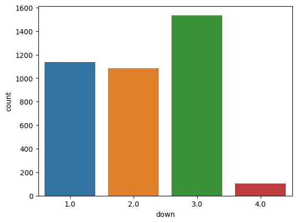
Third down has the highest number of sacks, which is intuitive since defenses often increase pressure in these higher-leverage situations, and offenses may take more risks with longer-developing plays to convert.
Sack Distribution by Number of Pass Rushers
The number of pass rushers sent by the defense is another important factor:
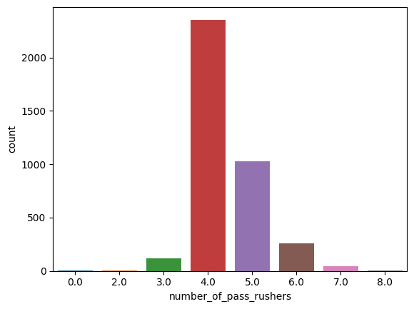
Interestingly, sending 4 pass rushers results in the highest number of sacks. This aligns with the NFL norm where teams often rush 4 and drop 7 into coverage, creating a balance between pressure and coverage.
Sack Distribution by Defenders in the Box
The number of defenders positioned in the box pre-snap can also indicate potential pressure:
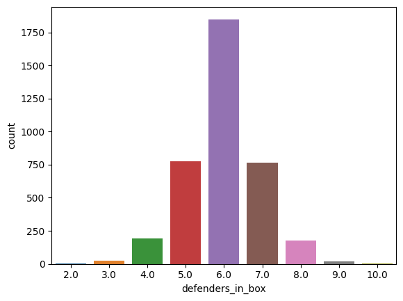
Having 6 defenders in the box is associated with the highest sack count, which provides insight into optimal defensive formations for generating pressure.
Logistic Regression Model
For our predictive model, we used logistic regression with the following features:
- Down (1st, 2nd, 3rd, 4th)
- Distance to first down
- Field position (yards to goal)
- Number of pass rushers
- Number of defenders in the box
- Score differential
- Time remaining in game
- Formation (shotgun vs under center)
# Create binary sack outcome variable
pbp_pass <- pbp %>%
  filter(play_type == "pass", !is.na(sack)) %>%
  mutate(sack_binary = as.factor(sack))

# Build logistic regression model
sack_model <- glm(
  sack_binary ~ down + ydstogo + yardline_100 + pass_rushers + defenders_in_box + score_differential + game_seconds_remaining + shotgun,
  data = pbp_pass,
  family = "binomial"
)

# Summary of model
summary(sack_model)
Model Results and Evaluation
The logistic regression model achieved reasonable predictive performance with an AUC (Area Under the ROC Curve) of 0.68, indicating moderate discriminative ability. The most significant predictors of sack probability were:
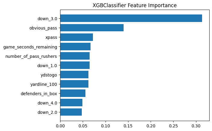
Key insights from the model:
- Down and distance are strong predictors, with third-and-long situations having higher sack probabilities
- Shotgun formation is associated with lower sack rates compared to under-center formations
- More defenders in the box increases sack probability, but with diminishing returns
- Game context matters - teams trailing late in games experience higher sack rates as they take more risks
Practical Applications
This model can be valuable for both offensive and defensive game planning:
- For offensive coordinators: Identify high-risk situations and adjust protection schemes accordingly
- For defensive coordinators: Recognize optimal blitz scenarios based on game situation
- For quarterbacks: Be more aware of pressure likelihood in specific situations
- For analysts: Evaluate offensive line and quarterback performance with context-adjusted metrics
Conclusion
Logistic regression provides a powerful tool for modeling sack probability in the NFL. While our model has moderate predictive power, it generates valuable insights into the factors that influence quarterback sacks. Future work could incorporate more granular data such as offensive line rankings, quarterback mobility metrics, or defensive personnel packages to further improve predictive accuracy.
Understanding these patterns can help teams optimize their strategies on both sides of the ball, potentially creating meaningful advantages in the highly competitive NFL landscape.