In the competitive world of NFL, play prediction has become increasingly important for defensive coordinators and analysts. In this post, I'll explore how Random Forest Classification can be used to predict whether the next play will be a run or pass based on game situation variables.
Understanding the Problem
Play-calling in the NFL is a complex decision influenced by numerous factors: down, distance to go, field position, score differential, time remaining, and more. If a defense can accurately anticipate the upcoming play type (run or pass), they gain a significant advantage.
While NFL coaches and coordinators have traditionally relied on tendencies, intuition, and basic statistics, machine learning offers an opportunity to identify more complex and subtle patterns in play-calling that might not be immediately apparent to human observers.
Data Collection and Preparation
For this analysis, I used the NFL play-by-play data from the 2020, 2021, and 2022 seasons, focusing on regular offensive plays (excluding special teams plays and no-plays).
import pandas as pd
import numpy as np
import matplotlib.pyplot as plt
import seaborn as sns
import nfl_data_py as nfl
from sklearn.ensemble import RandomForestClassifier
from sklearn.metrics import classification_report, confusion_matrix
from sklearn.model_selection import train_test_split

# Get data for 2020-2022 seasons
years = [2020, 2021, 2022]
pbp = nfl.import_pbp_data(years)

# Filter for standard plays (remove penalties, timeouts, etc.)
plays = pbp[(pbp['play_type'].isin(['pass', 'run'])) &
           (~pbp['play_type'].isin(['no_play', 'qb_kneel', 'qb_spike']))]
Feature Selection and Engineering
After examining available data, I selected and engineered the following features:
- Game situation variables: down, distance to go, yard line, quarter, time remaining
- Score dynamics: score differential, whether team is leading/trailing
- Derived features:
- "Obvious passing situation" (e.g., 3rd and long, trailing late)
- "Goal-to-go" situations
- Time pressure indicators (e.g., under 2 minutes in half)
# Create feature dataset
features = plays[['down', 'ydstogo', 'yardline_100', 'qtr', 'game_seconds_remaining',
                 'score_differential', 'goal_to_go']]

# Add derived features
features['obvious_pass'] = ((plays['down'] == 3) & (plays['ydstogo'] >= 7)) | \
                          ((plays['score_differential'] <= -10) & (plays['game_seconds_remaining'] <= 600))
features['under_two_min'] = (plays['qtr'].isin([2, 4])) & (plays['game_seconds_remaining'] % 1800 <= 120)
features['is_leading'] = plays['score_differential'] > 0

# Create target variable (1 for pass, 0 for run)
target = (plays['play_type'] == 'pass').astype(int)
Exploratory Data Analysis
Before building the model, I explored play type distributions across various situations:

The analysis revealed several expected patterns:
- Pass plays are more common on 3rd down (when teams typically need more yards)
- Teams trailing by 10+ points in the 4th quarter pass nearly 80% of the time
- Run plays are more common when leading in the 4th quarter (to run out the clock)
Random Forest Classification Model
I chose Random Forest Classification for this task because:
- It handles non-linear relationships well
- It's resistant to overfitting with proper tuning
- It provides feature importance measures
- It can capture complex interactions between variables
# Split data into training and testing sets
X_train, X_test, y_train, y_test = train_test_split(
    features, target, test_size=0.25, random_state=42
)

# Train Random Forest model
rf_model = RandomForestClassifier(
    n_estimators=100,
    max_depth=10,
    min_samples_split=10,
    random_state=42
)
rf_model.fit(X_train, y_train)

# Evaluate model
y_pred = rf_model.predict(X_test)
print(classification_report(y_test, y_pred))
Model Results and Evaluation
The Random Forest model achieved an overall accuracy of 69.4%, with balanced precision and recall for both play types:
| Play Type | Precision | Recall | F1-Score |
|---|---|---|---|
| Run (0) | 0.67 | 0.64 | 0.65 |
| Pass (1) | 0.71 | 0.74 | 0.72 |
The confusion matrix shows that the model correctly predicted:
- 64% of run plays (true negatives)
- 74% of pass plays (true positives)

Feature Importance Analysis
Examining feature importance reveals which variables most strongly influence play-calling decisions:
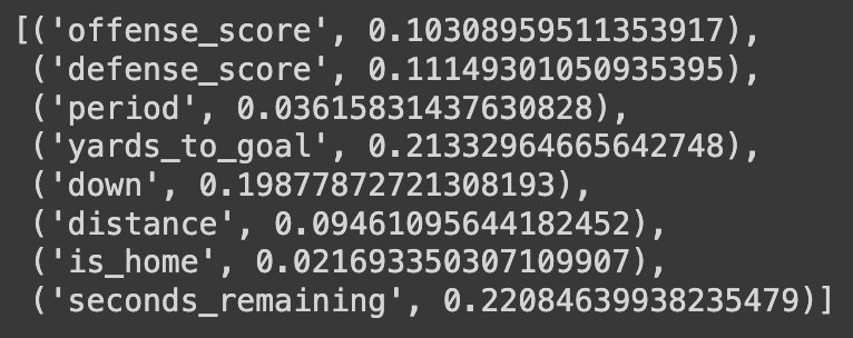
The most important features were:
- Down (28%): Particularly influential for 3rd downs
- Distance to go (19%): Longer distances favor passing plays
- Game seconds remaining (16%): Time pressure influences play-calling
- Score differential (12%): Teams trailing pass more often
- Yard line (11%): Field position affects risk tolerance
Practical Applications
This model could be valuable for:
- Defensive coordinators: Better anticipating offensive tendencies
- Offensive coaches: Identifying and avoiding predictable patterns
- Broadcasters and analysts: Providing data-driven insights during games
- Fantasy football players: Understanding situational tendencies for player projections
Team-Specific Models
To demonstrate how play-calling tendencies vary by team, I trained separate models for three teams with different offensive philosophies:

Interesting findings include:
- The Ravens were more run-heavy in all situations compared to league average
- The Chiefs showed higher passing rates on early downs
- The 49ers exhibited more balanced play-calling in most situations
Limitations and Future Improvements
While the model shows promising results, several limitations exist:
- It doesn't account for personnel packages or formations
- It lacks information on coaching tendencies or matchup specifics
- Weather conditions are not included as features
- It treats all teams the same (unless team-specific models are built)
Future improvements could include:
- Incorporating tracking data for formation and personnel identification
- Including coach and coordinator-specific tendencies
- Adding weather and field condition variables
- Implementing ensemble methods combining team-specific and global models
Conclusion
Random Forest Classification provides a powerful tool for predicting NFL play types based on game situation variables. With 69.4% accuracy, the model demonstrates that substantial information about play-calling decisions is contained in basic game state features.
While not perfect (and no model would be, given the intentional unpredictability of play-calling), this approach offers valuable insights into situational tendencies and could serve as a foundation for more sophisticated predictive models incorporating additional data sources.